How Maximum Power Point Tracking (MPPT) Works, Simplified

And implementing a perturb-and-observe (P&O) algorithm on an ESP32

What is MPPT?

Maximum Power Point Tracking is a technique used by solar inverters or power converters to maximize the power output from PV (photovoltaic) systems. The maximum power point is not static - it varies with irradiance and temperature of the solar panels, hence needing an algorithm to track these changes and adjust the load accordingly.

First principles: PV Cell Equivalent Circuit

An ideal PV cell can be abstracted as a current source with a diode connected in parallel.

In the ideal case, the series resistance will be zero, and the shunt resistances will be infinite. But in the real world, both the series and shunt resistances have finite values, and must be considered.

The generated current (I) by the PV cell can be seen on the right of the diagram below.

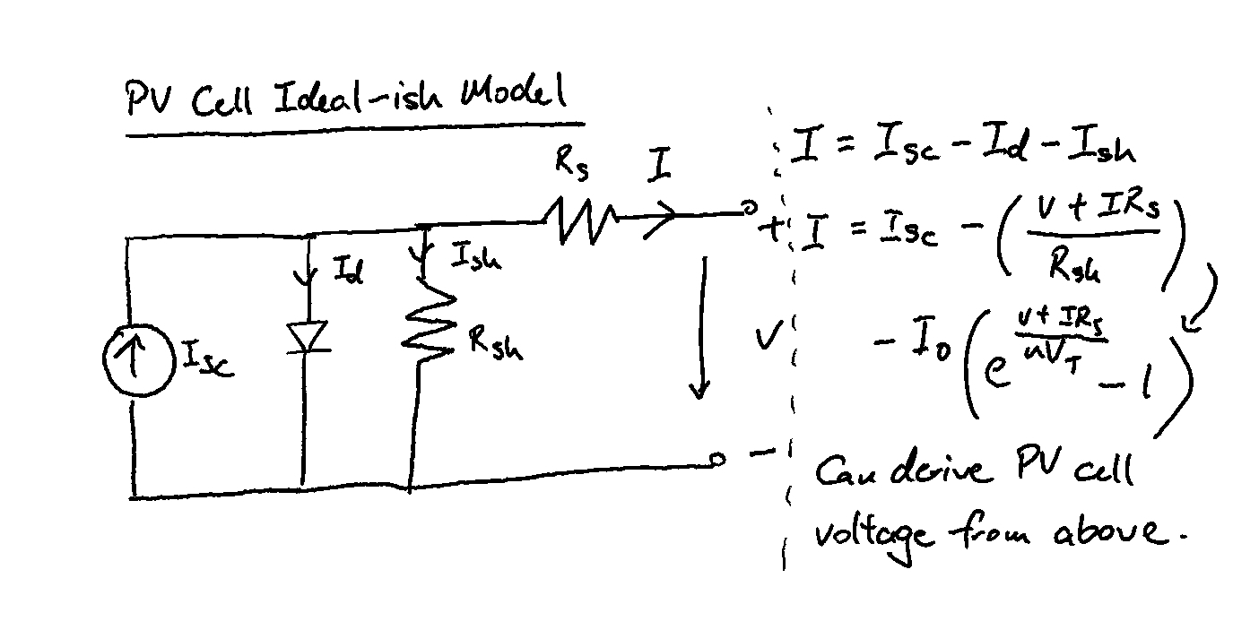
Where VT is the thermal voltage, Rs and Rsh are the internal series and parallel resistances respectively, Isc is the short-circuit current, Io is the reverse saturation current, VD is the voltage across the diode, I is the current output and n is the “ideality factor” of the diode.

PV Cell I-V Curve

Hence, PV cells have nonlinear I-V characteristics. As mentioned above, these characteristics change with irradiation levels and temperature.

In an I-V curve, the maximum power point is always at the knee of the curve (as seen below).

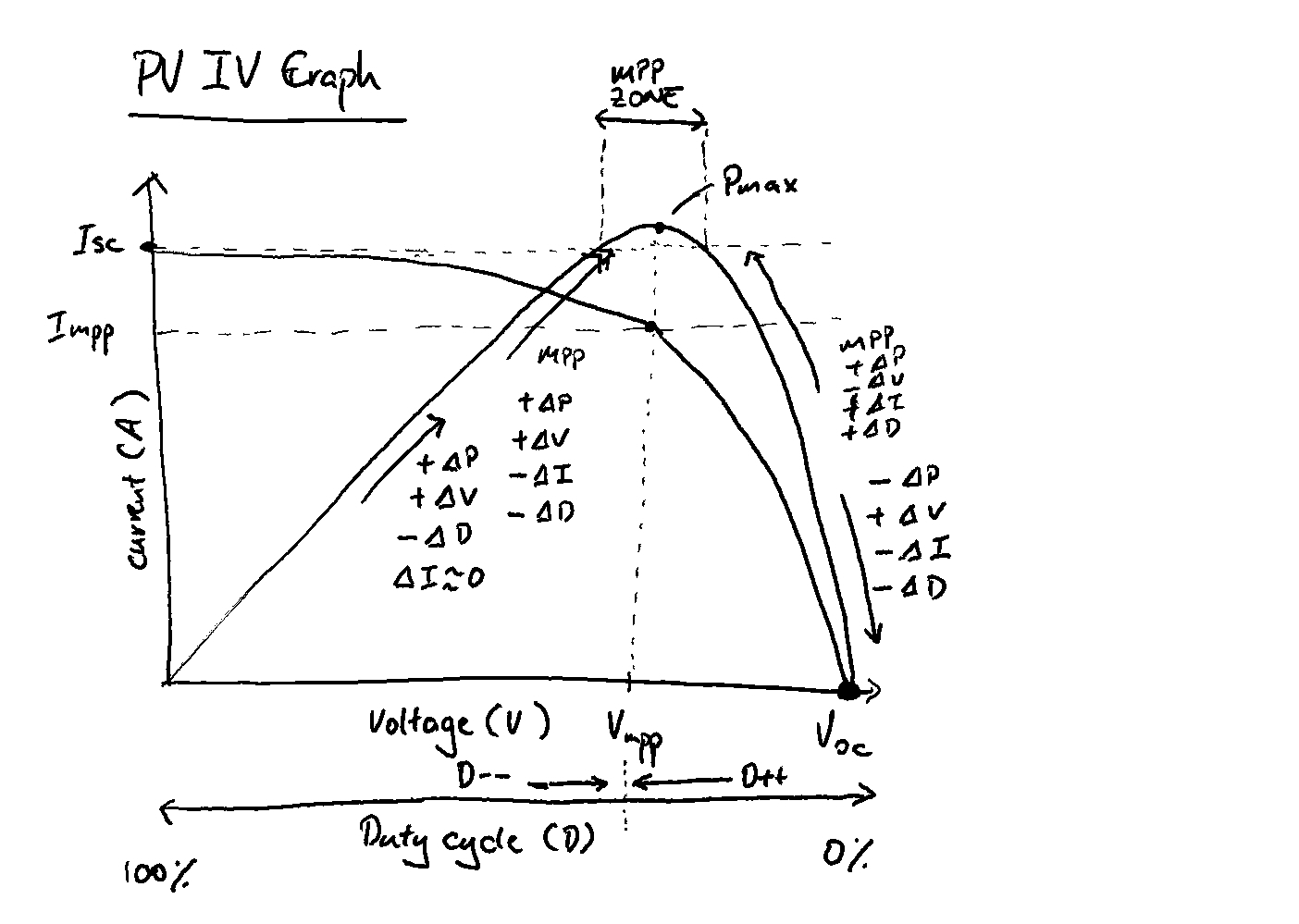
The above graph shows the current-voltage (I-V) characteristics of a typical silicon PV cell operating under normal conditions.

The power delivered by a single PV cell is the product of it’s output current and voltage (I x V = Power). If you were to follow, point for point, all the voltages (from short-circuit to open-circuit), you can visualize the power curve above for a given radiation level.

When the PV cell is open-circuited (i.e. not connected to any load), the current will be at it’s minimum (zero), and the voltage across the cell will be at it’s maximum. This is known as the PV cell’s open circuit voltage (Voc).

At the other extreme, when the PV cell is short-circuited (i.e. connecting the positive and negative leads directly together), the voltage across the cell is at it’s minimum (zero), and the current flowing out of the cell reaches it’s maximum. This is known as the PV cell’s short circuit current (Isc).

Of course, neither of these two conditions generate any electrical power (common sense, but also can derive from V x 0(I) or 0(V) x I). What’s interesting is all the in-between points where the PV cell generates power - and especially - the one particular combination of current and voltage for which power reaches it’s maximum value, at Impp and Pmpp. This is the maximum power point or MPP.

This is the I-V curve for a single PV cell. A PV panel is just made up of multiple PV cells interconnected together in series and parallel. Ipso facto, the I-V curve of a PV panel is just a scaled up version of the single PV cell I-V curve above.

Perturb & Observe algorithm

The Perturb & Observe algorithm operates on a simple principle: make small adjustments (perturbations) to the operating voltage and measure the resulting power output.

If the power increases, continue in that direction. If it decreases, reverse the direction. This makes sure that the system is constantly nudged towards peak power output. Think of it as a hill-climbing method.

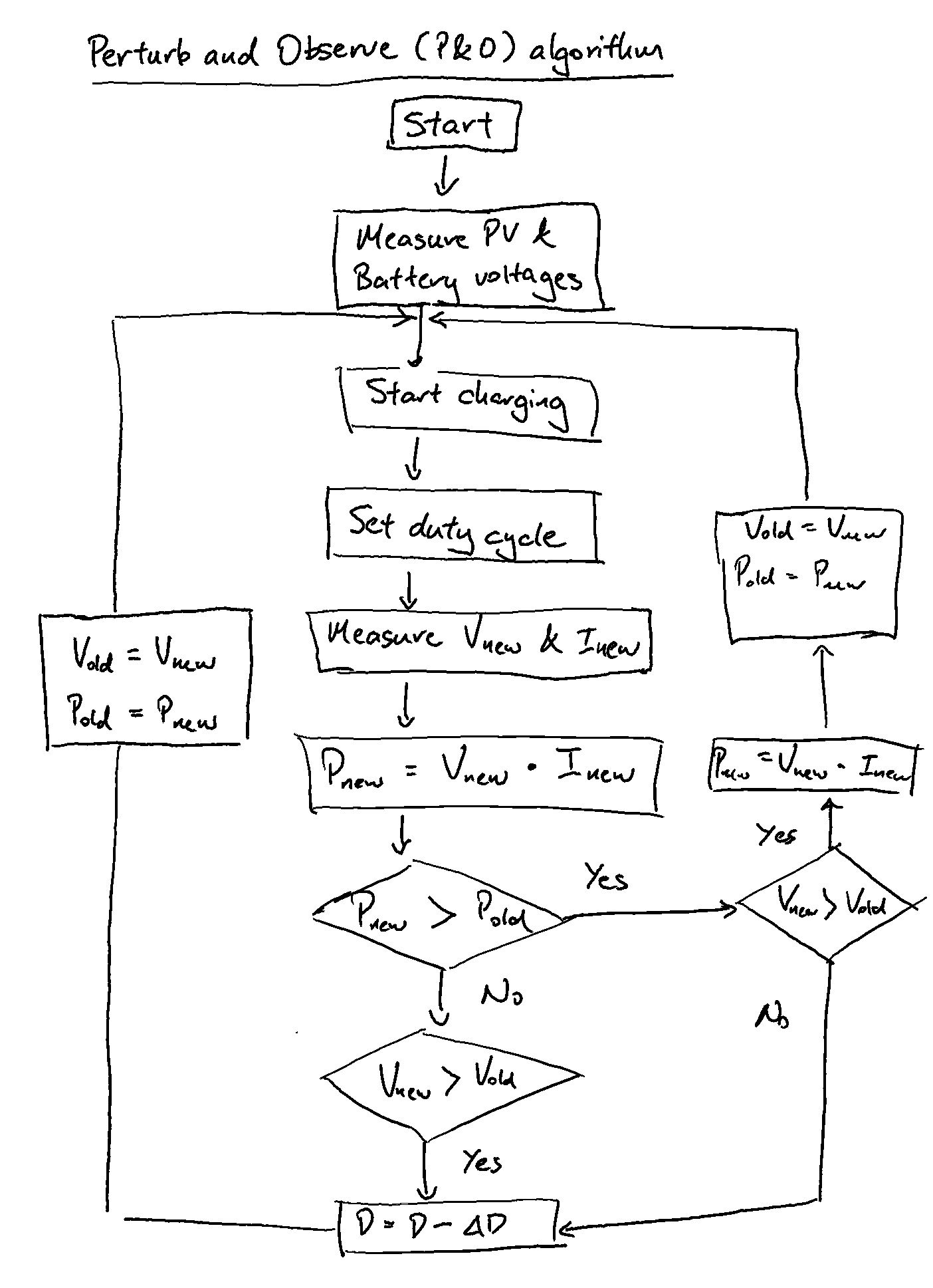
Here’s some pseudo-code for the above diagram:

Initialize:
    V_old = 0
    I_old = 0
    P_old = 0
    Delta_V = 0.1  // Arbitrary step size for voltage perturbation
    Duty_Cycle = 50% // Initial duty cycle for the DC/DC converter

Start:
    Measure V_new (PV voltage)
    Measure I_new (PV current)
    P_new = V_new * I_new // Calculate the new power

    If P_new > P_old:
        If V_new > V_old:
            Increase Duty_Cycle
        Else:
            Decrease Duty_Cycle
    Else:
        If V_new > V_old:
            Decrease Duty_Cycle
        Else:
            Increase Duty_Cycle

    V_old = V_new
    I_old = I_new
    P_old = P_new

    Wait for a short period (say ~9 ms)

    Repeat Start

It’s pretty straight-forward. You are controlling the duty cycle like a knob, which makes the power output seesaw back and forth a pseudo-equillibrum.

Hardware implementation

We decided to use the ESP32, which is a very fast and powerful 240MHz 32-bit dual core microcontroller, which costs less than $3 (with built in WiFi and Bluetooth!).

Having two cores is really sweet, because that allows us to run two independent processes. [1]

By allotting a dedicated core for the MPPT, we were able to get to 9ms per loop cycle.

The ESP32 has 16-bit Pulse-width Modulation (PWM) resolution, which also really helps in a buck converted based MPPT. The higher resolution, the finer the voltage and current steps. And we can also trade off “excess” PWM bit resolution for higher PWM frequency.

Traded off some PWM resolution for switching frequency, ending up with 11-bit PWM resolution and switching frequency of 39 kHz. [2]

Notes

[1] We don’t want to interfere with the crucial main MPPT algorithm (written in C++).

The MPPT algorithm regulates voltage and current - and could lead to unsafe operating conditions if gummed up. e.g. WiFi telemetry takes ~500ms of processing time to send. It would not be a good idea to combine it with main system processes.

[2] The ESP32 is blazing fast, considering it’s cost. Pretty cool.